Future Physics Projects in SAInT Center

A list of possible Physics related experiments that could be conducted in the SAInT Center

1. Find different types of conductors and insulators, and find the behaviour of these materials in the SEM. Since the SEM shoots high energy electrons at the sample, there is a potential difference which makes the sample light up differently when we observe it under the microscope. Goal is to calculate the conductivity of these elements, if possible, using the SEM.

2. Find a correlation between data of XRF HD Prime and SEM. SEM uses weight composition while the HD Prime uses counts (ppm). HD Prime discovers a lot more trace elements than the SEM, and SEM takes longer to analyze/quantify. Do research about the data correlation or contact Bruker/XOS.

Contacted Bruker and XOS to find out the correlation between the data. Very little or no data comparison was found online.

Comparing XRF and SEM can be found in the XOS website;

https://xos.com/technologies/sem/

Question that was asked:

Can we find a correlation between data of XRF HD Prime and SEM? SEM uses weight composition while the HD Prime uses counts (ppm). We do research for various samples using both the instruments the HD Prime and the SEM in the Saint Center in Siena College. Why would we choose the HD Prime over SEM for data analysis? How can we correlate the data between the instruments if we do use both instruments?

Awaiting a response.

3. AFM Spring Constants - The AFM uses a cantilever with a point on it that moves up and down. There is a spring attached to this cantilever and the different springs that are used in the AFM have different spring constants. This might be possible to analyze.

4. AFM Force - Look at the force correspondence between the cantilever and the sample pushing back on the cantilever. We can examine the graph on the screen to help with this analysis. The graph goes up and down in depending on the movement of the cantilever.

5. AFM Laser Diffraction - Find how the change in the angle of the cantilever affects the laser beam that is to be detected by the detector and how the AFM recognizes this change.

6. Maldie Instrument - Use the Maldie and calculate a particle's mass by accelerating it through a magnetic field and examining the radius of the circular path that the particle makes before it hits the detector. Therefore, determining the particle that was accelerated into the magnetic field.

7. Maldie test with hair sample to see if we are made with corn. (Dr. Finn)

8. Determine other Physics Projects that could be done in the SAInT Center using other instruments. (Brainstorm)

9. Get more Physics Students interested in SAInT Center Projects

Roger Bacon Physics Lounge

Dust was also collected in the Physics Lounge because the bookshelf was riddled with dust. There was so much dust that we believed that it would be possible to view the dust under the XRF. Below is the video of us collecting our first sample.As you can see we continue to use gloves while we collect our samples so that there is no chance of us contaminating it. A second sample was taken from the same place. 

Below is the image of the Sample 1 of the dust we had collected. We felt as a group that this would be a good location to begin analyzing the dust.

As you can see, most of the image was not filled by an element when it was analyzed. This means that they were most likely part of the Carbon tape, since we decided to exclude Carbon from our mapping. Sodium (Na), Aluminum (Al), Silicon (Si), Sulfur (S), Chlorine (Cl), Potassium (K), Calcium (Ca), Magnesium (Mg), Titanium (Ti), Iron (Fe), these were the elements found in the this dust sample. We believe that the Chlorine came from the cleaning materials used to clean the room. However, we are unsure of how it was able to get on top of the books.

This is the image along with the scanned elements that we found. This helps show that some of the part of the image were not comprised of the found elements. These elements do not include Oxygen and Carbon. The reason for this is that the tape is made of Carbon and the adhesive parts are Oxygen.

The spectrum was created so that we could analyze it to determine which elements were actually discovered. If an element was discovered, there would be a peak where the label is. However, if there is a label but no peak is visible then the element is not there.

We then quantified the elements to see how much of each element was there. This does not include Oxygen and Carbon as mentioned above. As you can see there is an abundant of Chlorine, Aluminium, and Calcium compared to the other elements.

Element	AN	series	[wt.%]	[norm. wt.%]	[norm. at.%]	Error in wt.% (1 Sigma)
Sodium	11	K-series	0.607596871	5.332369872	7.324763432	0.069220997
Magnesium	12	K-series	0.086324654	0.757599333	0.984355385	0.03144771
Aluminium	13	K-series	3.006961504	26.38958772	30.88686535	0.176977152
Silicon	14	K-series	1.799933455	15.79651144	17.76180058	0.106813871
Sulfur	16	K-series	0.812507693	7.130700878	7.022558956	0.056485865
Chlorine	17	K-series	1.910974947	16.7710298	14.93889168	0.092178816
Potassium	19	K-series	0.543853814	4.772950341	3.855112042	0.043151567
Calcium	20	K-series	1.986300483	17.43209907	13.73572564	0.084954204
Titanium	22	K-series	0.379779984	3.333011472	2.198318578	0.037302193
Iron	26	K-series	0.260266334	2.28414007	1.291608359	0.033623212
		Sum:	11.39449974	100	100

This is the area that we have decided to examine on Sample 2 under the SEM. 

After analyzing Sample 2, this is what was produced. The elements that were found in Sample 2 are identical to the ones found in Sample 1. This is good for us because this means that the data is consistent and there is no error in analyzing it. Of course Carbon and Oxygen were removed from the mapping. Even though the elements were consistent, the amount of them has clearly changed.

This is the elements with the image included so that you can see which part of the dust is composed of which element.

Just to make sure, we always examine the spectrum to check and make sure that each element is actually there, regardless of whether or not it was also found in the previous sample.

This is the data that we received after quantifying our spectrum. As you can see the composition of the dust is fairly similar to Sample 1. As mentioned above, Oxygen and Carbon have been removed.

Element	AN	series	[wt.%]	[norm. wt.%]	[norm. at.%]	Error in wt.% (1 Sigma)
Sodium	11	K-series	0.517404959	4.981322117	6.98322161	0.063236732
Magnesium	12	K-series	0.062626548	0.602937798	0.799507808	0.030033728
Aluminium	13	K-series	2.130154776	20.50808929	24.49651424	0.133178361
Silicon	14	K-series	1.443314914	13.89553072	15.94552428	0.090874711
Sulfur	16	K-series	1.187609971	11.43372848	11.49182254	0.070279841
Chlorine	17	K-series	1.960704124	18.87670121	17.16021048	0.09392205
Potassium	19	K-series	0.642771159	6.188286632	5.101035797	0.046257543
Calcium	20	K-series	1.911645311	18.40438693	14.79998035	0.082858875
Titanium	22	K-series	0.296168543	2.85136601	1.919307901	0.035047571
Iron	26	K-series	0.234499938	2.257650811	1.302874988	0.033009373
		Sum:	10.38690024	100	100

An issue that occurred while attempting to use the XRF on the dust is that the layer was too thin to get accurate data from it. This was the first place that there was an abundance of dust that a clump of it was collected.  Unfortunately the abundance of dust turned out to be useless.


Tristen Protzmann Prepping to place the Carbon tape onto the plate so that it can be examined under the SEM.

Dirt Samples in Wet Willy's [Car Wash]

Another location that we obtained dirt from is the Wet Willy's cash wash which is located at 701 New Loudon Rd, Latham, NY 12110. Our intention was to find something interesting compared to the set of elements we generally analyzed. The dirt sample was wet and so to remove all the moisture trapped in the dirt, it needed to be dried up in the oven. 

As usual, the dirt sample was analyzed in both the SEM and the HD Prime.

The raw image of the section of the dirt sample that was analyzed in the SEM is shown bellow;

The lighter shade particles that can be seen in the sample above represents the large particles of dirt.

The sample was analyzed for 9 minutes in the EDS to get better results of the element composition. The following results was obtained for the elemental mapping of the sample. The following picture also contains a outline of the raw image shown above. As usual, each element is represented in different colors.

The result that was obtained was more clear than the raw image itself and the small dirt particles can be seen as well. Note that Carbon and Oxygen are neglected in analyzing the sample for elemental compositon.

The new elements that were traced were Cadmium and Manganese.

The map of elemental composition itself is shown;

The spreadsheet data that was obtained after quantifying for weight composition of the dirt sample is shown below;

Element	AN	series	[wt.%]	[norm. wt.%]	[norm. at.%]	Error in wt.% (1 Sigma)
Sodium	11	K-series	0.517452789	1.307357089	1.79880694	0.062543746
Magnesium	12	K-series	0.685729394	1.732512035	2.254787351	0.065966061
Aluminium	13	K-series	5.332921697	13.47375672	15.79599263	0.292948185
Silicon	14	K-series	22.5837991	57.05851916	64.26333962	1.02922487
Phosphorus	15	K-series	0.174544453	0.440990816	0.450360788	0.033684536
Sulfur	16	K-series	0.054706279	0.138216748	0.136345508	0.02809259
Calcium	20	K-series	2.620305254	6.620265123	5.225096264	0.103002426
Titanium	22	K-series	0.515898718	1.303430691	0.861110244	0.040437744
Manganese	25	K-series	0.048569741	0.122712636	0.070654755	0.027262929
Iron	26	K-series	5.741094516	14.5050153	8.215675883	0.171269138
Cadmium	48	L-series	1.305043287	3.29722369	0.927830017	0.06695208
		Sum:	39.58006523	100	100

The most amount of weight composition that was found in the dirt sample was Silicon with a weight percentage of 57.1%. This is expected to be there because of the sand. A significant amount of Aluminium, Calcium and Iron can be seen with a weight percentage of 13.5%, 6.62% and 14.5% respectively.

The spectrum of the elements that were found in the same sample is shown below;

The amount of elements in the dirt sample can be seen in the spectrum using the peaks.

The results for the data that was obtained from analyzing the sample in the HD Prime is shown below.

Recall from the previous blog post...

...The cam view (wide view, Side view) of the sample is included in the data. The row of elements after the view shows the common elements that are expected to be seen in the sample. However to get a accurate results, we should look into the full results table shown in the second image. We will be looking into the counts column in this part to identify the elements with the most amount of counts that were detected...

Using the HD Prime, a excessive amount of Chromium was seen to be found using the list of elements shown after the side/wide view. This is seen using the red outline in the general list of elements that is found. To confirm this first look, we can look into the full results that can be seen in the second image.

 611.9 counts were measured for Chromium which is not a lot but still a consistent amount for a heavy metal.

Chromium is a lustrous, brittle, hard metal. Its color is silver-gray and it can be highly polished. It is mainly used in stainless steel, chrome plating and metal ceramics. It is also used to impart corrosion resistance and a shiny finish; as dyes and paints, its salts color glass an emerald green and it is used to produce synthetic rubies; as a catalyst in dyeing and in the tanning of leather.

Hence finding it in a Car wash can be completely understood but still a frequent level of exposure is advised to be avoided.

Other elements such as strontium, Iron, Copper, Titanium and Zinc was analyzed to be in the sample with counts exceeding 1500 counts. However these elements are not known to be hazardous.

References;

http://www.lenntech.com/periodic/elements/cr.htm

Old Hoffman's Playland Dirt Sample

A dirt sample was collected from the old Hoffman's playland. We thought it would be interesting because it is now abandoned and there was a lot of traffic and machinery over the years on the land. Here's our picture of the dirt from the SEM.


The next image is an elemental analysis map, without the map overlapping the image. The second picture is with SEM image in background.




Below is the spectrum from the elemental analysis and the quantified data.




After Carbon and Oxygen were removed from the data we see that the sample was more than half Silicon. The interesting elements we found were Titanium, and Indium. Although not much of these elements were present in the sample. Indium can sometimes be toxic and Titanium is a valuable metal. Below you can see the information from the XRF.


The XRF portrays a different outcome from its elemental analysis and shows us that the sample is primarily Iron and the SEM informed us that only about %10 of the sample was Iron. Not sure which to go off of, but we are more interested in finding rare or hazardous elements. In this sample there we no dangerous amounts of any toxic elements and very few amounts of rare, valuable elements. So we can conclude that the dirt around the old  Hoffman's Playland is quite bland. Below you can see Asaph Ko and Tristen Protzmann working with the dirt by the SEM.

Differential Scanning Calorimetry

 A Differential Scanning Calorimetry (DSC) is a thermoanalytical technique in which difference in the amount of heat required to increase the temperature of a sample and reference is measured as a function of temperature. The DSC takes from 30 minutes to 90 minutes to complete one full measurements.The special thing about this instrument is that it is a reversible process. Below is a picture of this instrument.

Below is the 3D Printer where we took filament samples from. After using the DSC we are capable of knowing when the filament undergoes a phase change. We then can program the 3D Printer to know when this phase chance occurs, and account for it when printing.

Below are some images of processes and tools needed to prep a sample to be tested in the DSC.

Below is a picture of our research group with Dr. Kolonko working with the DSC.

After being trained on the DSC our group was able to operate the DSC on our own. Below is a picture of our research group analyzing our first sample.

Below is a picture of Tristen Protzmann prepping our 3D Printer Filament to be analyzed in the DSC. The sample must be really small and has to fit in a pan to go into the DSC. After cutting it and measuring it, the sample was approximately 4.6mg.

We used the scale below to measure the weight of this sample.We use this scale only for when we are operating the DSC. It is very sensitive and precise with its measurements. 

Below is a picture of the DSC Pan Press. We use it to forcibly attach the pan lid to the pan with our sample inside the pan. Once the lid is on tight we can put it into the DSC and analyze the sample. 

Below is a picture of how we organized our samples for the DSC. We put each sample into a pill holder and labeled each slot. We then recorded it on the paper corresponding to its slot.

Below are the tools needed to press the pan lids onto the pan. As you can see there are various sizes to use when preforming this task. We mainly used the biggest black attachment located at the bottom of the third column (going from left to right).

Below is a picture of the pans we used, as well as, the pan lids. They are Tzero Pans. They weigh about 50mg each.

Below are the types of 3D Printer Filaments that we researched using the DSC. We took samples of filaments around the campus to expand our limits. We took samples from the SAInT Center, Dr. McColgan's Office, Roger Bacon 121, and the Stack Center. We found that all these filaments are PLA and would not release any toxic material when analyzing. 

Below are all our data collections from our research on the Blue 3D Printer Filament:

Below is the data collections from testing the Blue Polystyrene 3D Printer Filament. We set the Differential Scanning Calorimeter (DSC) to the Cool, Heat Cool setting. This means that the DSC cools the sample first. It then proceeds to heat up the sample to locate the phase change where the solid state of the filament transforms into the gooey liquid state that we need. The DSC helps us to locate and analyze when and where this phase change occurs. Once we know this we can program the 3D Printer to account for it. By knowing the specific temperature needed to melt the filament, we can set the tray of the 3D Printer to know when and how to heat up the filament to make it gooey enough to mold the object, as well as, when to cool it so the operator can take the object off once it is done printing. In the first picture we can see the linear relationships of how the sample is changing in the DSC as time progresses. In the second picture we have zoomed into the spot in the data where the actual phase change occurs. We can see the phase change occurs between 103°C and 108°C. This was a successful data collection.

Below is our second data collection. This time we used Purple ABS 3D Printer Filament. We did the same Cool, Heat, Cool setting for this sample. The same procedure was done for this sample. Below we can see the phase change occurs between 106°C and 109°C. This sample data collection was also very successful. 

SAInT Center Instruments

Here is a collection of pictures we took over the duration of our research in the SAInT Center. Below will be brief explanations of each picture and instrument shown.

Above is a picture of the tools we used to begin our research. The following tools can be seen: Gloves, Pen, Carbon Tape, Paper Towels, 3 Different Sized Stages, 2 Different Shaped Tweezers, Scalpel, Scissors, 3D Printer Filament, Stage Holder, Dirt Container, Beaker, and Acetone. Acetone is used to clean the stages after we are done using them. Adhesive Carbon Tape is used to collect our dust samples. The Dirt Container is used to look at our dirt samples under the XRF. The Tweezers and Scalpel are used to load our samples onto the stages. The Stage and Stage Holder get loaded into the SEM when ready to take data collections. Gloves are always worn to make sure we do not contaminate the samples. The Glass Beaker is used to put the dirt samples into the oven to dry them out. A Pen is always needed to record our data. Scissors are needed to cut the 3D Filament which we analyze in the DSC and TGA. Paper Towels are used to clean up our work station after we conclude our research for the day.  

As our research continued more tools were added. Above we can see a few. Plastic Wrap is needed to cover the dirt samples when placed in the XRF. This is because the XRF cannot be in direct contact with the samples, so plastic wrap is needed to make sure they do not touch. When we analyze samples that are not dirt in the XRF we use the Square Plastic Cover. It is flat and smooth and makes sure our samples do not come in contact with the XRF tip. Tape is used to label our samples, as well as, tape the plastic wrap on them to keep them from moving. A Scrapper is needed to help clean our stages and make sure the carbon tape is completely removed from the stages. Safety goggles can also be added to this list of materials. Safety goggles are mandatory and must be worn at all times when in the SAInT Center.

Above is an image of the inside of the SEM, as well as, the process of loading the SEM. Notice the "CAUTION X-RAYS" Warning Label. When handling samples gloves are always needed.

 When loading the stage, the X and Y Coordinates must always be set to 20-20. This can be seen in the image above. This centers the stage so when we load and EVAC the SEM the sample will be ready to view. It also prevents the stage from hitting the top, bottom, or sides of the SEM when loading the samples. The X-Y knobs are used to move the electron beam around the sample and navigate the stage around the inside of the SEM.

Above is a picture of our main work station. This is a picture of the Scanning Electron Microscope (SEM). The monitors are used to see inside the SEM, and obtain our data.

Above is the Scanning Electron Microscope (SEM). It's a Hitachi SEM and has a Bruker attachment that will be explained later on. A SEM is a type of electron microscope that produces images of a sample by scanning it with a focused beam of electrons. The electrons interact with atoms in the sample, producing various signals that contain information about the sample's surface topography and composition. CAUTION: It releases x-rays.

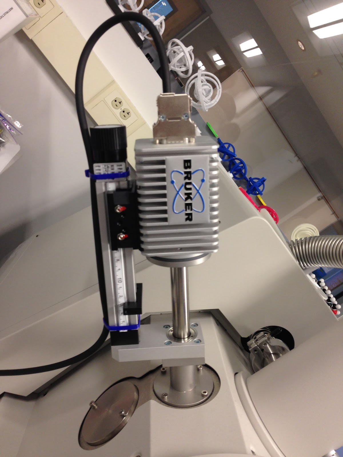
Above is a picture of the Bruker Attachment that is attached to the SEM. Bruker offers a powerful range of systems of Energy-Dispersive (EDS) and Wavelength-Dispersive (WDS) X-Ray Spectrometry Electron Backscatter Diffraction Analysis (EBSD), as well as, Micro-X-Ray Flourescence and micro computed tomography on the electron microscope. It is a valuable asset to our SEM Research.

Above is the left monitor we use for the SEM. Here we use the various knobs below the screen to adjust and perfect our images. The knobs are used for the adjustment of magnification, contrast, brightness, coarse and fine focus, and X-Y alignments. These help us to operate around the sample, and find a perfect location to analyze. This is always the first step in analyzing the samples in the SEM.

The image above is of the right monitor. On this monitor is where we can analyze and quantify our data. This is where we do most of our data collection, and how we discover the elements in our samples. The image has to be loaded over from the left monitor. Once it's loaded over we can do our data analysis and collections.

Above is an image of the inside of the SEM. On the side of the SEM there is a camera to see inside the SEM to help the operator navigate around. This is a little monitor located under the bigger monitors and has to be turned on and off manually. This camera CANNOT be On when using the right monitor and collecting data. It will skew our data completely and it not good for the camera. This camera is really helpful because once the SEM is vacuum sealed there is no way of seeing into the SEM without this camera. 

Above is a picture of the X-Ray Fluorescent (XRF) also known as the HD Prime. We use this machine along with the SEM to help us identify elements in our samples. The XRF identifies more elements than the SEM, and is beneficial for our research. A vacuum is needed over the HD Prime when operating because it releases radioactive material gases that need to be sucked out of the room to protect the operator from potentially dangerous gases. CAUTION: It releases x-rays.

Above is an image of one of the three ceiling vacuums in the SAInT Center. They suck in any airborne gases that may be released from machines or experiments that we may not be able to smell or see. This protects the researchers in the room from inhaling or in-taking any potentially dangerous gases. We placed the vacuum over the TGA and XRF when operating. 

Above is a picture of the Differential Scanning Calorimeter (DSC). A DSC is a thermoanalytical technique in which difference in the amount of heat required to increase the temperature of a sample and reference is measured as a function of temperature. The DSC takes from 30 minutes to 90 minutes to complete one full measurements. This machine is different from the TGA because it is reversible, meaning the sample can be cooled, heated, and re-cooled. This means the sample can have 2 separate phase changes from solid to liquid and back to solid. 

Above is the Refrigerator Cooling System that is attached to the DSC. This cools the DSC when necessary and helps our samples to complete 2 phase changes. This is beneficial because it helps us heat up and cool a sample when we need to. This is essential when we do our 3D Filament samples.  

Above is a picture of a scale we use to weigh our samples and their pans. We use this scale only for when we are operating the TGA and DSC. It is very sensitive and precise with its measurements. 

Above is the 3D Printer that is located in the SAInT Center. We used the filament from this printer in the DSC and TGA experiements. The 3D Printer is able to melt plastic filaments and mold them into a 3 dimensional object on its heated bed.

Above is a Thermogravimetric Analyzer (TGA). The TGA is used as a method of thermal analysis in which changes in physical and chemical properties of materials are measured as a function of increasing temperature (with constant heating rate), or as a fucntion of time (with constant temperature and/or constant mass loss). This machine takes about 45 minutes to an hour to make one successful measurement. Notice that for this machine it is imperative to use bronze tweezers over your regular aluminium or steel. Also, it is important to use the ceiling vacuums over this machine when operating. Once the phase change is complete with this machine the process is irreversible. 

Above is a picture of the Oven we used to heat up and dehydrate our dirt samples. It fluctuates between 104°F and 106.5°F and we left each sample in around an hour. This is important because if any water is found in our samples when placed in the SEM it could either damage the SEM or ruin our sample. 

Above is a picture of the fume hood we used when cleaning our stages. The purpose of the hood is to extract all chemical gases or fumes that may be emitted from the acetone when cleaning the stages.

Above is a picture of the DSC Pan Press. We use it to forcibly attach the pan lid to the pan with our sample inside the pan. Once the lid is on tight we can put it into the DSC and analyze the sample. 

Above is a picture of an Atomic-Force Microscope (AFM). An AFM is a very high resolution type of scanning probe microscopy (SPM), with demonstrated resolution on the order of fractions of a nanometer, more than 1,000 times better than the optical diffraction limit. We have not used this machine yet by ourselves, but we plan to once we have undergone more training. We plan on doing more experiments with Graphene once we are. The first picture is the AFM itself, while the picture below it is where we conduct the experiments on the AFM. We have only ran one experiment with the AFM, and that data can be found in the Graphene blog.

*(Some definitions of the instruments were researched with the help of Wikipedia.com)*